Satellite Data Features
衛星データでできること

土地の肥沃度、石油残量、夜の地球の明るさを人工衛星から観測し、その状況と変化から農作物収量、石油備蓄量、GDPなどを予測することができます。
衛星データビジネスを知る
衛星データから駐車場の車両台数をカウントし、企業の業績予想を算出するとともに、これを指標化し株価予測に役立てている例もあります。
衛星データビジネスを知る
広範囲な森林を人工衛星により効率的に観測し、樹種分類による森林管理や病害虫の被害把握などが行われています。
衛星データビジネスを知る世界の物流の約9割を占める海上輸送では、衛星による航路のトラッキングや違法漁船の位置データ等を把握することで、海上保険や海難救助に役立てられています。
衛星データビジネスを知る
海面水温、植物性プランクトン、海面高度などの情報による魚群探査が行われています。また、水産養殖でも環境データとしてリスク解析に活用されています。
衛星データビジネスを知る
衛星データから農作物の作付面積、生育状況、食味の把握や適期収穫時期の予測を行い、農業生産者の生産性と収益性を向上する意思決定支援が行われています。
衛星データビジネスを知る- 資産調査
- 株価予測
- 森林監査・管理
- 物流
- 魚群探査・養殖監視
- 農作物の生育予測
いつでも、どこでも、だれでも、 手軽にデータを扱える世界に。
Product Features
Tellus サービスラインナップ

- 衛星データ
-
国内外の政府衛星・商用衛星のデータを取り揃えています。
衛星データ一覧をみる

- 地上データ
-
衛星データと組み合わせて活用方法が広がります。
地上データ一覧をみる

- ツールのAPI提供
-
データの前処理や解析に利用できます。
ツール一覧をみる


- 衛星のシーン検索
-
Tellus Travelerで探す


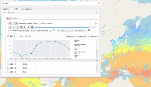
- 開発/解析環境
-
開発/解析環境をみる

For Your Business
Tellusを使ってビジネスをしたい方
Tellusでは共にビジネスを創造するパートナーを探しています。衛星データの新しい可能性をTellusとともに創出しましょう。
SORABATAKE
学ぶ・知る Pick up記事(宙畑)
- 2026/02/05 メンテナンス システムメンテナンスのお知らせ(02/12 14:00-15:00)
- 2025/12/11 ニュース 年末年始における問い合わせ窓口の対応について
- 2025/12/11 ニュース 一部地上データ提供終了のお知らせ
- 2025/11/20 メンテナンス システムメンテナンスのお知らせ(11/27 15:00-15:30)
- 2025/11/13 ニュース 【国内初】衛星データ活用、法人向けクラウド型ワークスペース「Tellus Pro」提供開始!