Introduction

Satellite images are not much different to simple photographs captured from the air without performing appropriate reading analysis on the acquired satellite images. We can acquire useful images by reading images after learning how to interpret and analyze satellite images.

4.1 Basics of Image Interpretation

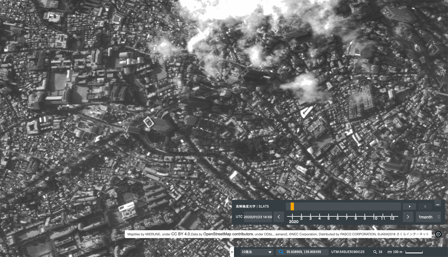
Interpreting satellite images involves capturing elements such as tones, shapes, sizes (scales), patterns, textures, shadows and association (relatedness) that are the visual elements of different targets.

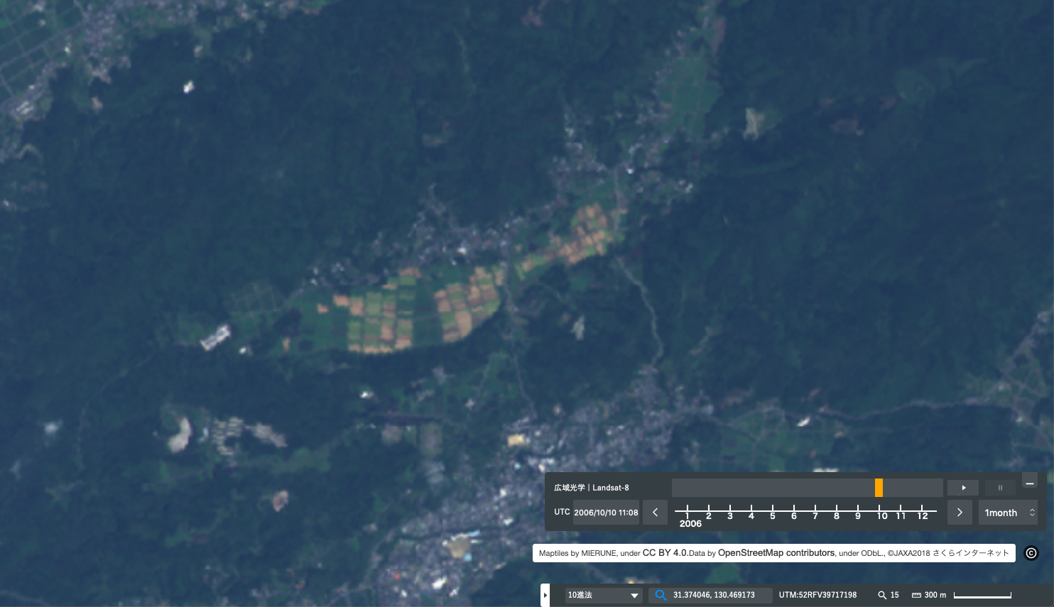
Tone: The tone refers to the brightness or color of images. The tone is a basic element to distinguish various targets or different features.

Shape: The shape indicates the structure or outline of each target. Linear shapes are typical of man-made objects. This applies to houses and fields. On the other hand, natural objects have more complicated shapes.

Size or scale: The size of the target in an image is important in estimating how big it is in reality.

Pattern: A pattern represents the spatial arrangement of the target. The repetition of similar tones and textures becomes a pattern that can be identified as a specific feature.

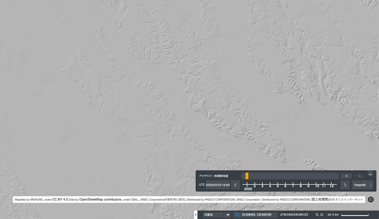
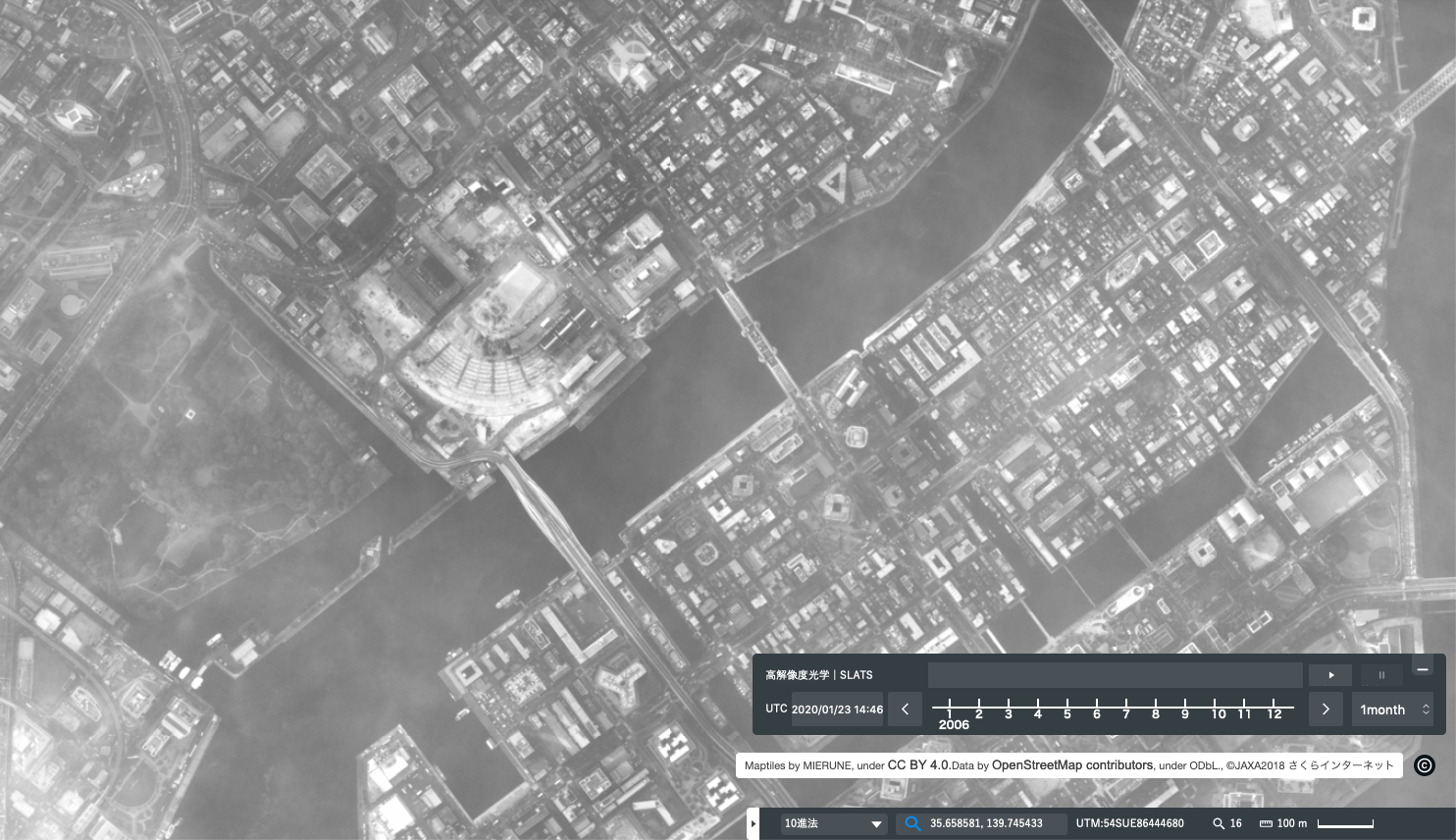
Texture: The texture indicates the distribution and frequency of color tone changes in specific regions in an image. A rough texture consists of a mottled pattern because the tone changes dramatically over a small range. On the other hand, a smooth texture is represented with a smooth surface because the changes in tone are extremely scarce.

Shadow: Shadows provide information relating to the height of the target. On the other hand, those shadows obscure other targets.

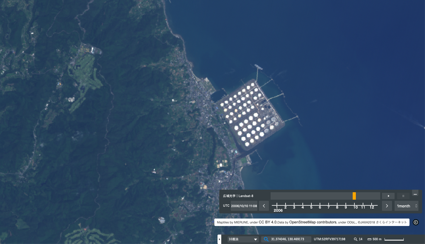
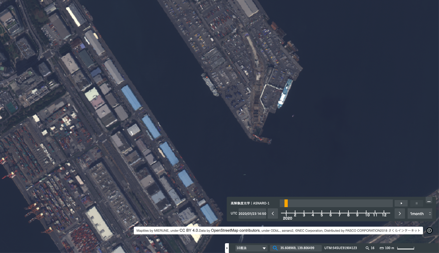
Association: Association shows the relatedness between the target and objects or features in its proximity. Considering the connections with other features helps to interpret the target. For example, large commercial facilities, industrial areas, containers, wide roads and similar are associated with reclaimed land.

4.2 Digital Image Processing

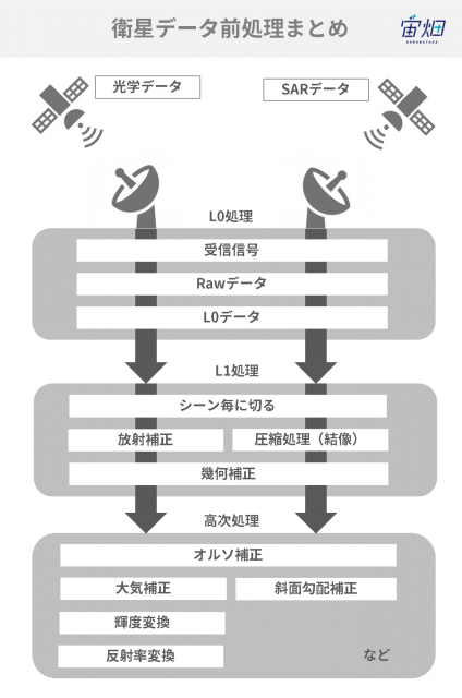
Pre-processing: This includes radiometric correction or geometric correction and is performed before the main analysis. L0 processing in the first process is the processing first performed after data is received from the satellite. If we look closely at L0 processing, we can see three steps:

(1) Radio waves from satellites are received by antennas on the ground

(2) The received signals are processed for transmission, so are returned to their original signals (raw data)

(3) Unnecessary information is deleted from the raw data (L0 data)

The satellite data in the L0 stage is data that ordinary people rarely look at. Therefore, please think of this as processing performed in the company or organization that owns the satellite.

・Image correction: This improves the appearance of the image. It helps with interpreting and analyzing the image.

・Image transformation: Arithmetic processing (sum, difference, product and quotient) is performed to combine the original data obtained from each band into a single image. In addition, it is possible to eliminate excess information in hyperspectral data and to depict images efficiently through advanced calculations such as of the main components.

・Image classification and analysis: Images are classified into unsupervised images, supervised images and object-based image analysis (OBIA).

4.3 Preprocessing

Preprocessing transforms data into data closer to the scene in reality by correcting radiometric and geometric data distortions derived from sensors and platforms.

Preprocessing is classified into radiometric and geometric correction in general. We refer to L1 processing in particular here.

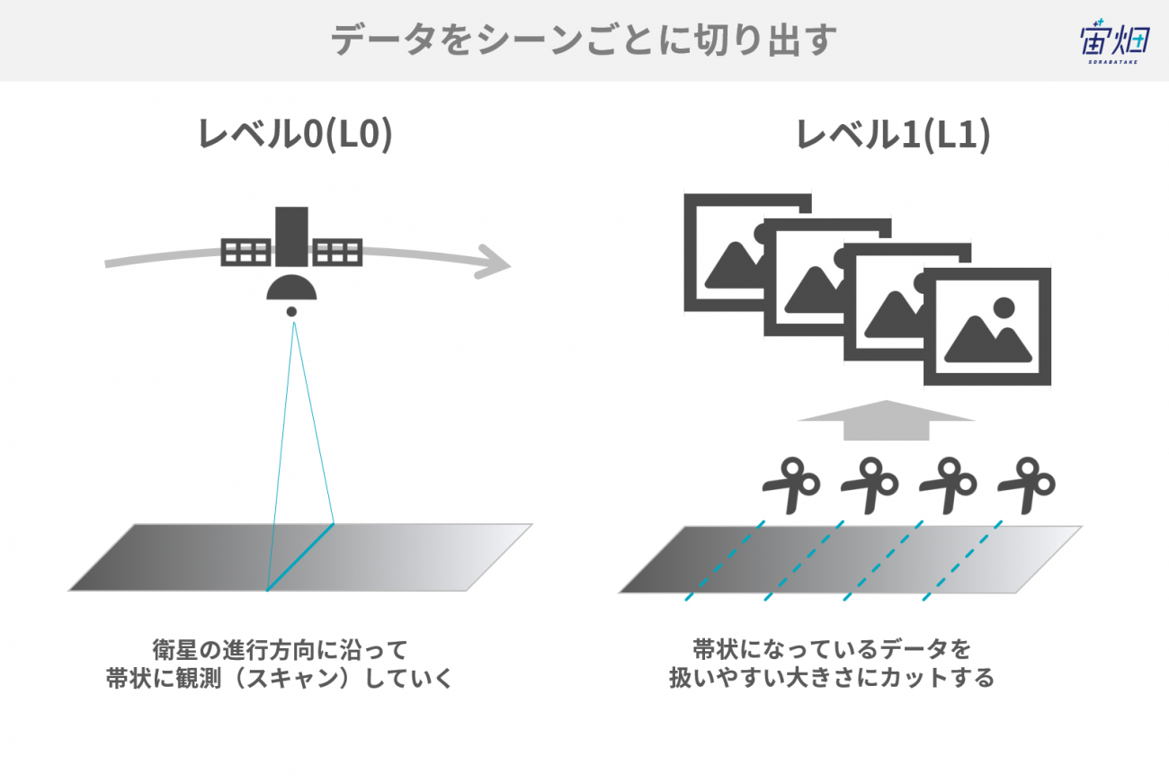
We can broadly divide L1 processing into three stages:

(1) Extraction for each scene

(2) Image sensitivity adjustment / imaging and creation of a picture

(3) Removal of image distortion

Satellites possess data for which the ground has been scanned in the direction of movement. This is data that is difficult to handle as it is (e.g., there are problems with the data capacity). Therefore, the data is reduced to a size that is considered appropriate. This is the work of cutting the data for each scene.

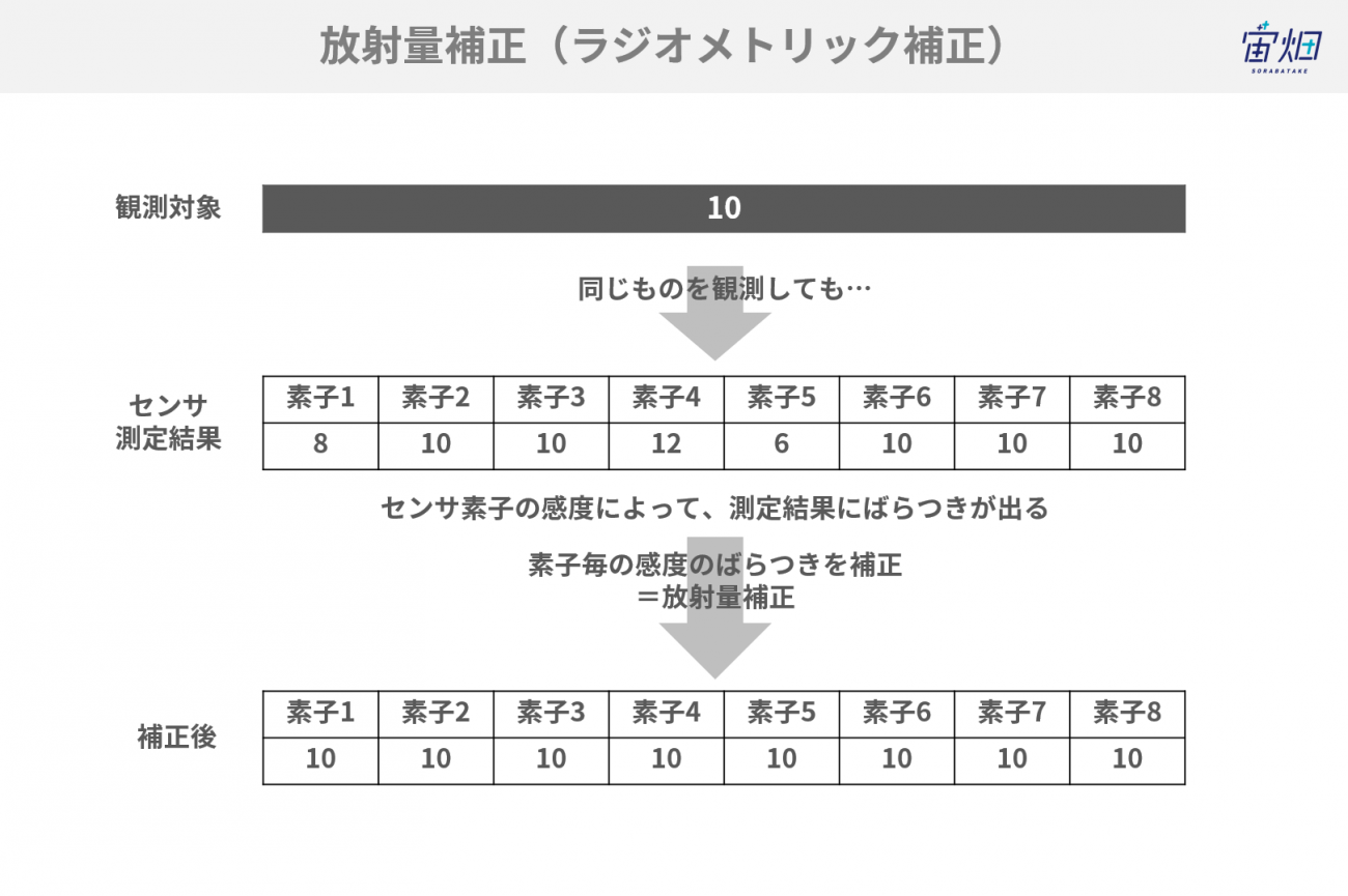
The processing performed next is called radiometric correction. The compression correction corrects the noise derived from the sensors and platforms and the noise in the atmosphere to accurately indicate the energy reflected or emitted as measured by the sensor. Simply speaking, this is work to clean up images.

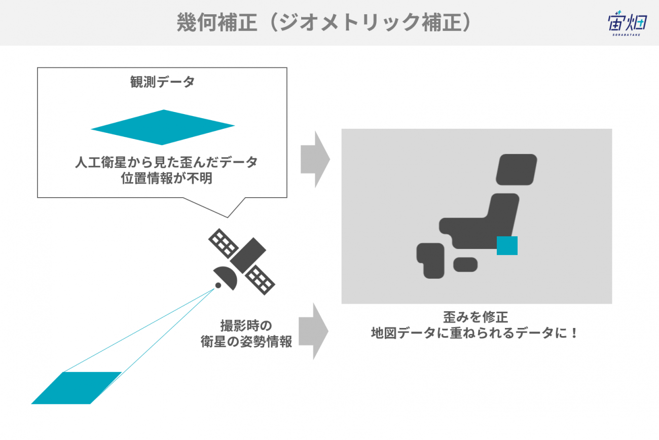
Geometric correction corrects the geometric distortions that are caused by geometric changes in the sensor and the earth. The data is replaced with the coordinates of the earth’s surface. (This is to transform it so that it precisely overlaps onto maps.

The following are considered.

・Coordinate changes

・Sensor height and capture speed

・Curvature of the earth

・Atmospheric refraction

・Image distortions (relief displacement)

・Nonlinearities in the sweep of a sensor’s IFOV

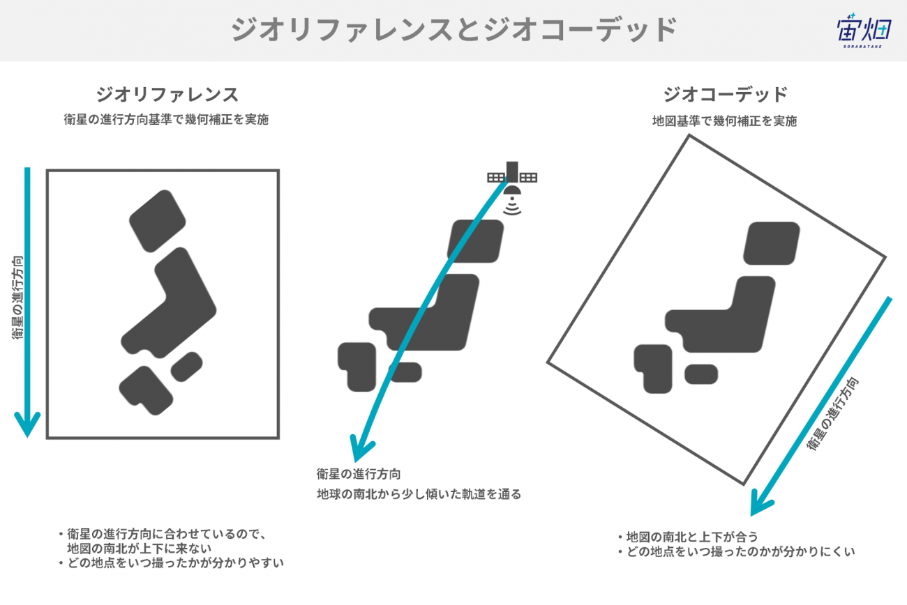
There are two ways of overlaying images on a map with geometric correction.

・Georeferencing: This is conversion to appropriately convert images to the actual coordinates

・Geocoding： All the pixels of an image are correctly placed in the coordinate system in the terrain

4.4 Post-processing

Re-sampling

Calculating the values of new pixels from the pixel values of the original image is called re-sampling. Re-sampling is performed when aligning and re-arranging image pixels onto map projections in post-processing. Raster data used in GIS is similar to photographs with color information in each cell. However, this does not mean that all cells have the correct value. (This is also called “empty” image pixels.) Therefore, it is necessary to fill in blank cells based on accurate color information

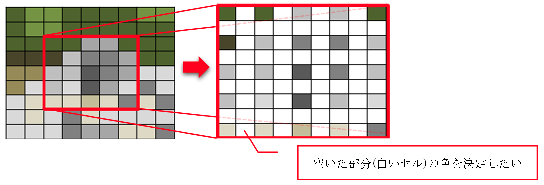
*Figure taken from https://www.esrij.com/gis-guide/imagery/resampling/

The typical calculation methods are nearest neighborhood, bilinear interolation and cubic convolution.

Nearest neighborhood：

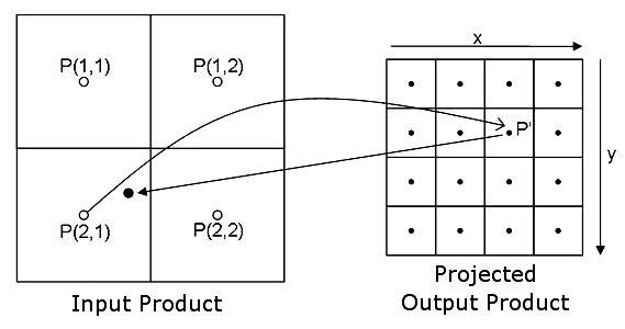
・The pixel values of a position close to the pixel coordinates of the result image and input image (original) are referenced in nearest neighborhood re-sampling.

・The original pixel values are not changed. However, some pixel values are duplicated or removed.

・The spectral information is accurate compared to other methods with this method. Therefore, it is suitable for when handling the spectral field. In addition, it is also a calculation method frequently used in the scientific field in which accurate spectral information is viewed as important.

https://www.brockmann-consult.de/beam/doc/help/general/ResamplingMethods.html

Bi-linear interpolation：

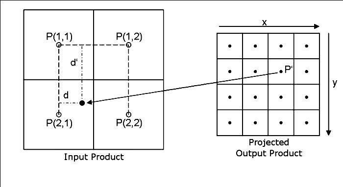
・The four pixels closet to the position (P’) of the pixel value in the figure on the left (the raster data of the results you wish to re-sample) are chosen from the input images and a weighted average value of those is taken.

・The original pixel values are changed in this method to create images with completely new pixel values.

・The pixel values are obtained with P’(x,y) = P(1,1)(1-d)(1-d’)+P(1,2)d(1-d’)+P(2,1)d’(1-d)+p(2,2)dd.

https://www.brockmann-consult.de/beam/doc/help/general/ResamplingMethods.html

Cubic convolution：

・This method involves selecting from the original image 16 pixels from a place close to the pixel value of the corrected image and then taking a weighted average value of those.

・The edges in the image are cleared up with bi-linear.

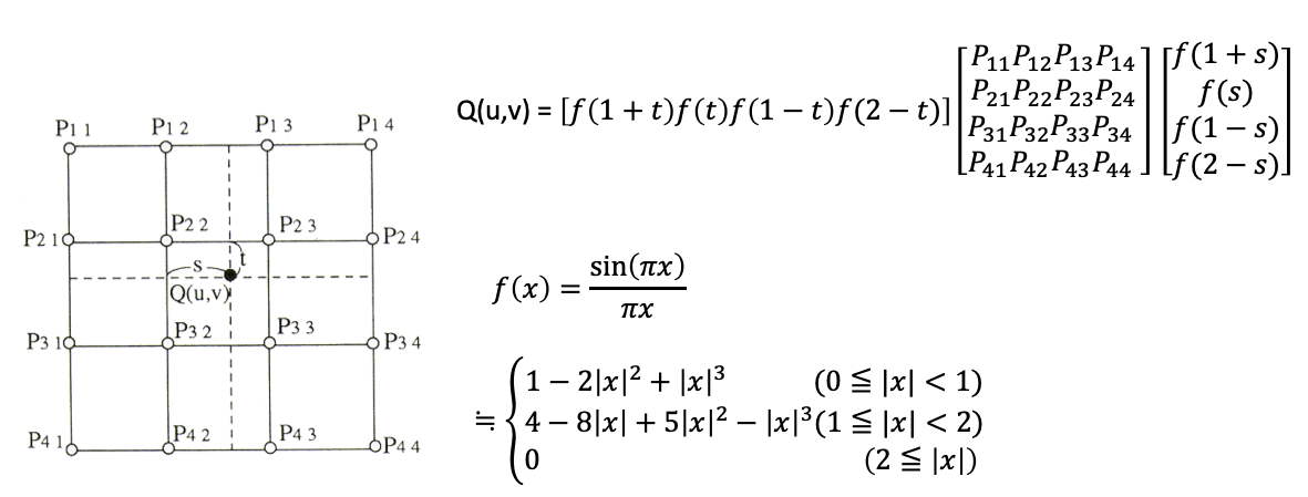
*The x is the difference between the coordinate (u,v) at the re-sampling point and the position (i,j) in the pixels of the input image
Source：http://wtlab.iis.u-tokyo.ac.jp/wataru/lecture/rsgis/rsnote/cp9/cp9-7.htm

The Q (u,v) at this time is the re-sampling point while the Pij is the pixel position of the input image.

Image enhancement

Image enhancement edits images to transform them into even easier-to-see images. Many enhancement effects lead to a distortion of the original data.

Contrast enhancement：

・Contrast enhancement also includes an increase in the contrast between the target and its background.

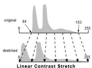
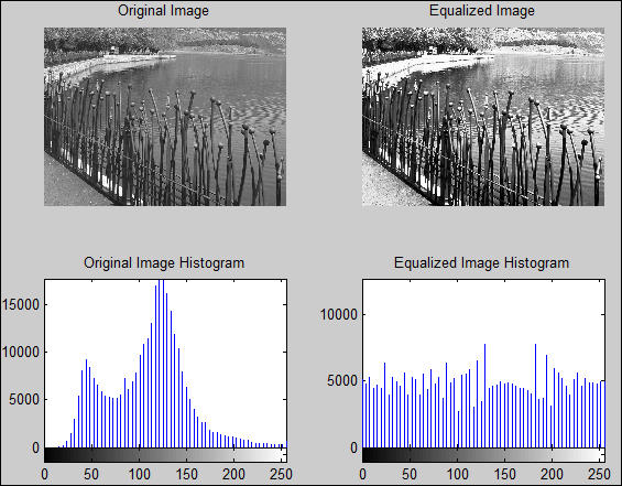
・It is very important to understand the image histogram concept to understand concept enhancement.

・An image histogram is a histogram that expresses the clearness of the values comprising the image.

・A histogram is created from the data in linear contrast stretch to obtain the upper and lower limits. This range is extended to the smallest and largest values as data (0 is the smallest value and 255 is the largest value in RGB).

Source：http://gis.humboldt.edu/OLM/Courses/GSP_216_Online/lesson4-2/radiometric.html

The histogram obtained from the original data is transformed into a flat histogram through a calculation instead of simply extending it to the smallest and largest values like with linear contrast stretch in histogram-equalized stretch.

Source：https://subscription.packtpub.com/book/hardware_and_creative/9781849697200/2/ch02lvl1sec24/histogram-equalization-for-contrast-enhancement

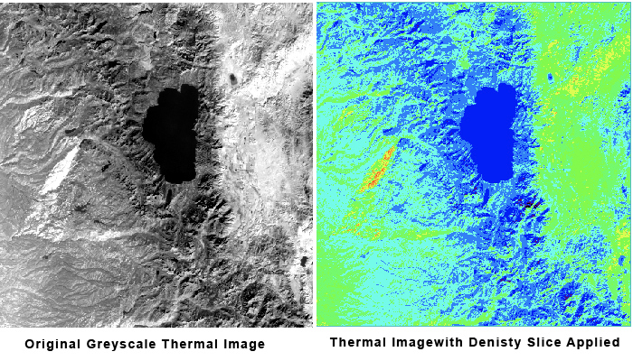
Density slicing：

・The digital values distributed on the x-axis of the image histogram are divided into specific intervals.

・Colors are assigned to each section (slice).

・This method is used for images that only have one band information. For example, if the temperature is divided into intervals of two degrees Celsius on a black and white thermal image, there is a color scheme according to each section. With this, it becomes easier to understand the temperature information than by looking at it in black and white.

Source：http://gis.humboldt.edu/OLM/Courses/GSP_216_Online/lesson4-2/radiometric.html

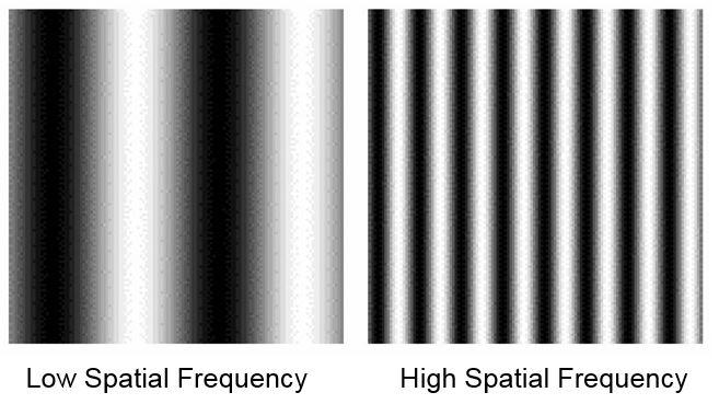
Spatial filtering：

・Specific things in the image are emphasized or suppressed based on the spatial frequency.

・The spatial frequency indicates the frequency of changes in tone in the image.

・The tone changes dramatically in a small area for rough textures. In this case, the spatial frequencies become higher. Meanwhile, if smooth, the spatial frequencies become lower.

Sources：http://gsp.humboldt.edu/olm_2016/courses/GSP_216_Online/lesson4-2/spatial.html

Source：http://gsp.humboldt.edu/olm_2016/courses/GSP_216_Online/lesson4-2/spatial.html

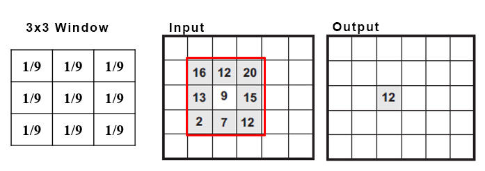
Low pass filters: This is a method of smoothing outliers by averaging the neighboring high and low values. Low pass filters are used to remove noise and to suppress local changes. The pixel values output are obtained by multiplying the coefficient acquired from the pixel values existing in the area surrounding it. This method is also one called convolution.

Image Classification and Analysis

Image classification involves classifying images using statistical methods based on the characteristic information contained in images. Image classification is roughly divided into unsupervised image classification and supervised image classification.

Unsupervised image classification:

The following steps are following in unsupervised image classification:

1. Generate a cluster
2. Apply to a class

For example, Iterative Self-Organizing Data Analysis (ISODATA) is a method in which spectral distance is used to cluster repeating pixels. Values are classified in unsupervised classification. However, no judgment is given about what that classification is. For example, after classifying into vegetation and non-vegetation, the analyst himself or herself must decide which is more appropriate as the cluster representing vegetation. Accordingly, it is difficult to accurately give meaning to clusters if the person performing the analysis does not have knowledge about the target area.

Supervised image classification:

There are three basic steps to this.

1. Select the training data (area selection) and generate the signature file
2. Classify
3. Output the results

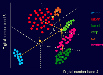
Extract the optimal image that represents the class from among the images and use that as the training data. For example, let’s say you will classify the images by water, sand, forest, urban area, cultivated land and grassland. The training data you have collected is brought together as a signature file. The classification is then performed according to the maximum-likelihood method and the support vector machine (SVM) from the target images using the signature files you have collected.

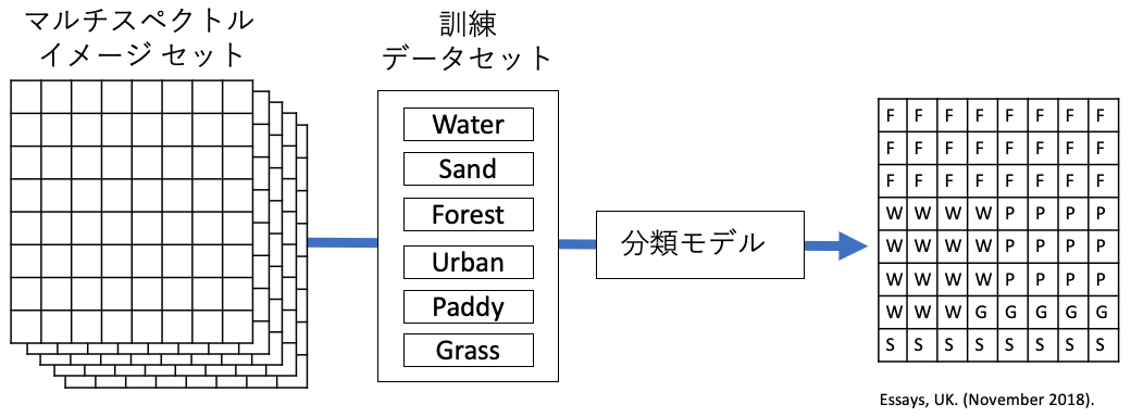
(1) Training: Establish the optimal training area and acquire the spectral data that will be the reference for the class. This information is used when creating the classification model as training data.

(2) Classification: All the pixels in the image are classified according to the model into the classes determined above. If it is determined that a pixel value does not belong to any class, it may be labeled as unclassifiable.

Source：International Journal of Computing and Network Technology Oil Spill Hyperspectral Data Analysis:
Using Minimum Distance and Binary Encoding Algorithms

(3) Output: In addition to being display on a map, the output of the results may be displayed as a table.

Supervised/unsupervised classification is a pixel-based classification. However, the grouped pixels are converted into vectors using an image segmentation algorithm in OBIA. The acquired objects are classified by spectral and spatial measures. This has the following meaning.

・Images are segmented into objects that capture the actual characteristics of the features in segmentation.

・Segmented objects are classified using shapes, sizes and spatial/spectral attributes in classification.

References:

・ Digital Image Processing | Natural Resources Canada

・ Image Classification Techniques in Remote Sensing

・ Digital Image Classification | GEOG 480: Exploring Imagery and Elevation Data in GIS Applications

・ Digital Image Calssification

・ How to Interpret a Satellite Image: Five Tips and Strategies

・ Remote Sensing Image Processing

・ BEAM Help - Resampling Methods